Recipes

ziggurat

Foresight.ziggurat Function

ziggurat(x; kwargs...)

Plots a histogram with a transparent fill.

Key attributes:

linecolor = automatic: Sets the color of the step outline.

color = @inherit patchcolor: Color of the interior fill.

fillalpha = 0.5: Transparency of the interior fill.

filternan = true: Whether to remove NaN values from the data before plotting.

Plot type

The plot type alias for the ziggurat function is Ziggurat.

source

x = randn(100)
ziggurat(x)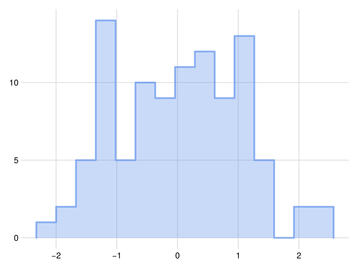

hill

Foresight.hill Function

hill(x; kwargs...)

Plots a density with a transparent fill.

Key attributes:

color = @inherit patchcolor: Color of the interior fill.

fillalpha = 0.5: Transparency of the interior fill.

filternan = true: Whether to remove NaN values from the data before plotting.

strokecolor = automatic: Color of the outline stroke.

strokewidth = 1: Width of the outline stroke.

Plot type

The plot type alias for the hill function is Hill.

source

x = randn(100)
hill(x)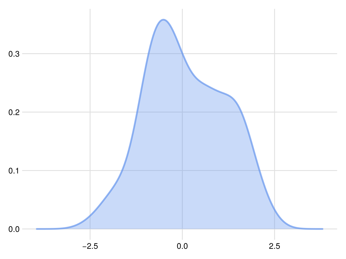

bandwidth

Foresight.bandwidth Function

bandwidth(x, y; kwargs...)

Plots a band of a certain width about a center line.

Key attributes:

bandwidth = 1: Vertical width of the band in data space. Can be a vector of length(x).

direction = :x: The direction of the band, either :x or :y.

Plot type

The plot type alias for the bandwidth function is Bandwidth.

source

x = -π:0.1:π
bandwidth(x, sin.(x); bandwidth = sin.(x))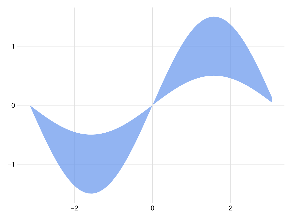

polarhist

Foresight.polarhist Function

polarhist(x; kwargs...)

Plots a polar histogram of the values in x. Attributes are shared with Makie.Hist and Makie.Poly.

Plot type

The plot type alias for the polarhist function is PolarHist.

source

polarhist(randn(1000) .* 2)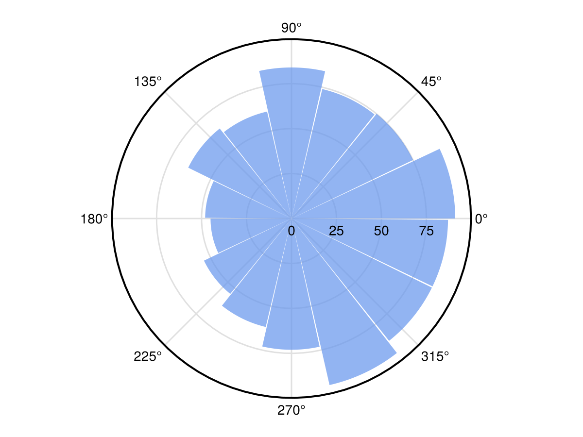

polardensity

Foresight.polardensity Function

polardensity(x; kwargs...)

Plots a polar density plot of the values in x.

Key attributes:

bandwidth = default_bandwidth_circular(x): The bandwidth of the kernel density estimate.

strokecolor = :density:

Sets the color of the stroke around the density band. Can be a color, or one of the following color modes:

• :density uses the density values as the color.

• :angle or :phase uses the angle of the values as the color.

• :transparent uses a transparent color.

Plot type

The plot type alias for the polardensity function is PolarDensity.

source

polardensity(randn(1000) .* 2;
                 strokewidth = 5,
                 strokecolor = :angle,
                 strokecolormap = cyclic,
                 colormap=:viridis)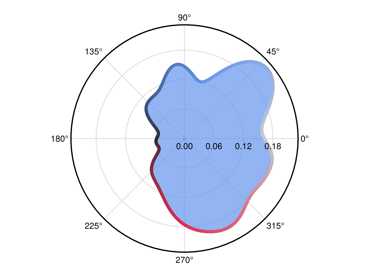

covellipse

Foresight.covellipse Function

covellipse(μ, Σ²; kwargs...)

Plots an ellipse representing a multivariate normal distribution with mean μ and covariance matrix Σ².

Key attributes:

scale = 2: The scale factor for the ellipse size, in units of standard deviation.

vertices = 1000: The number of vertices to use for the ellipse, or a list of angular vertices.

Plot type

The plot type alias for the covellipse function is CovEllipse.

source

xy = randn(100, 2) * [1 1; 0 0.5]
μ = mean(xy, dims = 1)
Σ² = cov(xy)

fig, ax, plt = covellipse(μ, Σ²)
scatter!(ax, xy)
fig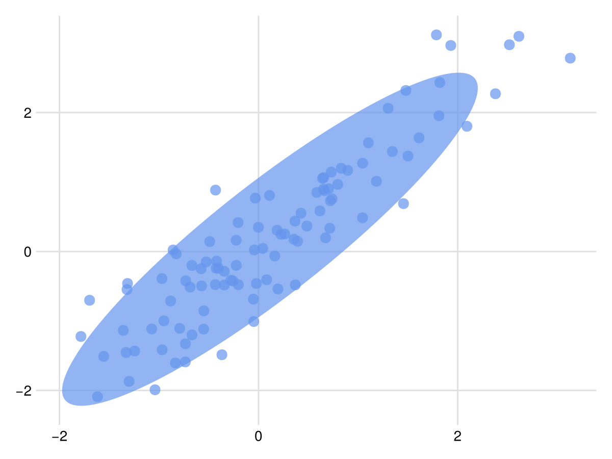

prism

Foresight.prism Function

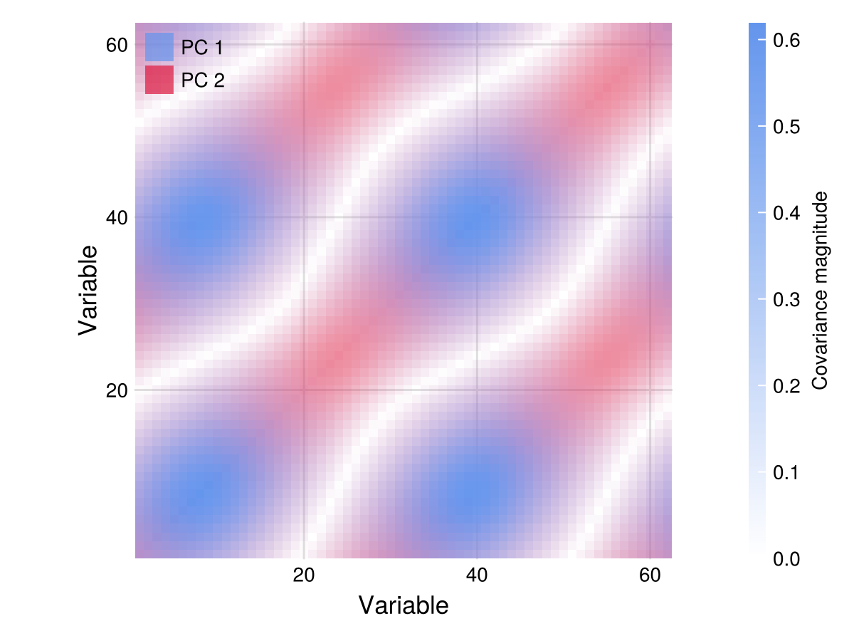
prism(x, Y; [palette=[:cornflowerblue, :crimson, :cucumber], colormode=:top, verbose=false.])

Color a covariance matrix each element's contribution to each of the top k principal components, where k is the length of the supplied color palette (defaults to the number of principal component weights given). Provide as positional arguments a vector x of N row names and an N×N covariance matrix Y.

Keyword Arguments

• palette: a vector containing a color for each principal component.

• colormode: how to color the covariance matrix. :raw gives no coloring by principal components, :top is a combination of the top three PC colors (default) and :all is a combination of all PC colors, where PCN = :black if N > length(palette).

• verbose: whether to print the feature weights to the console

source

ys = sin.((0:0.001:(π * 1.5)) .+ (0.1:0.1:(2π))')
Σ² = cov(ys .+ randn(size(ys)) ./ 10; dims = 1)
H = prism(Σ²; palette = [cornflowerblue, crimson]) # Generates the prism colors

f = Figure()
limits = (0, maximum(abs.(Σ²))) # You must set the limits manually
g, ax = prismplot!(f[1, 1], H; limits, colorbarlabel = "Covariance magnitude")
axislegend(ax,
            [
                PolyElement(color = (cornflowerblue, 0.7)),
                PolyElement(color = (crimson, 0.7))
            ],
            ["PC 1", "PC 2"], position = :lt)
ax.xlabel = ax.ylabel = "Variable"
f